WhipperSnapPy Tutorial

This notebook demonstrates static and interactive 3D brain surface visualization using WhipperSnapPy. It covers single-view snapshots (snap1), four-view overview images (snap4), and interactive WebGL rendering (plot3d).

Tutorial data from the Rhineland Study (Koch et al.), Zenodo: https://doi.org/10.5281/zenodo.11186582, CC BY 4.0.

Subject Directory

Set sdir to your own FreeSurfer subject directory. If you leave it empty, the sample subject sub-rs (one anonymized subject from the Rhineland Study) is downloaded automatically (~20 MB, cached locally after the first run).

import os

from whippersnappy import fetch_sample_subject

# Set sdir to your FreeSurfer subject directory.
# Leave empty ("") to automatically use the sample subject (sub-rs,
# one anonymized subject from the Rhineland Study). It is used directly
# from the repository when available, otherwise downloaded (~20 MB) and
# cached locally after the first run.
sdir = ""
# sdir = "/path/to/your/subject"

if not sdir:
    sdir = fetch_sample_subject()["sdir"]

print("Subject directory:", sdir)

Subject directory: /home/runner/.cache/whippersnappy/sub-rs

Derive file paths from sdir

All paths are constructed from sdir, so switching between subjects only requires changing the single variable above.

# Surfaces
lh_white     = os.path.join(sdir, "surf", "lh.white")
rh_white     = os.path.join(sdir, "surf", "rh.white")

# Curvature
lh_curv      = os.path.join(sdir, "surf", "lh.curv")
rh_curv      = os.path.join(sdir, "surf", "rh.curv")

# Thickness overlay
lh_thickness = os.path.join(sdir, "surf", "lh.thickness")
rh_thickness = os.path.join(sdir, "surf", "rh.thickness")

# Cortex label (mask for overlay)
lh_label     = os.path.join(sdir, "label", "lh.cortex.label")
rh_label     = os.path.join(sdir, "label", "rh.cortex.label")

# Parcellation annotation (DKTatlas)
lh_annot     = os.path.join(sdir, "label", "lh.aparc.DKTatlas.mapped.annot")
rh_annot     = os.path.join(sdir, "label", "rh.aparc.DKTatlas.mapped.annot")

snap1 — Basic Single View

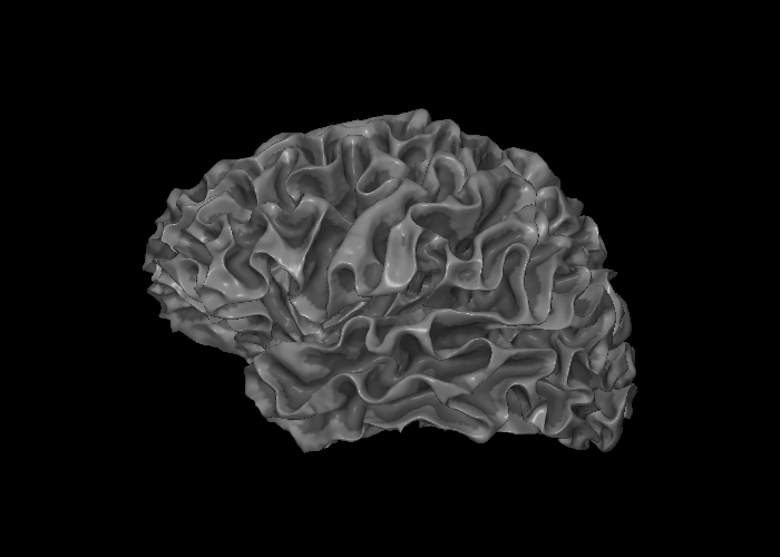
snap1 renders a single static view of a surface mesh into a PIL Image. Here we render the left hemisphere with curvature texturing only (no overlay), which gives the classic sulcal depth shading.

from IPython.display import display

from whippersnappy import snap1

img = snap1(lh_white, bg_map=lh_curv)
display(img)

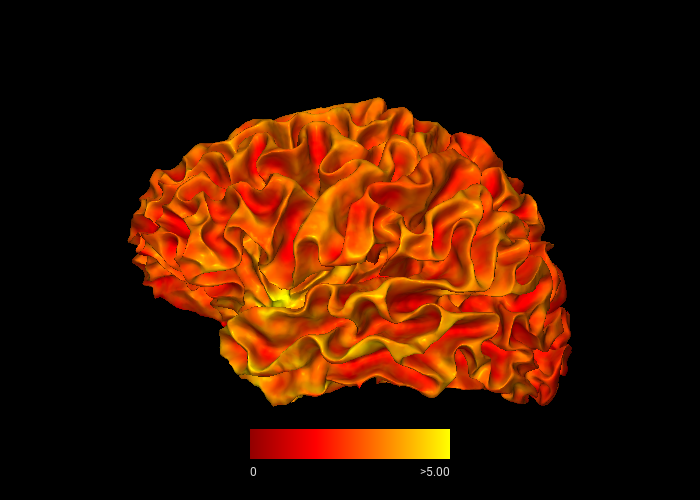
snap1 — With Thickness Overlay

By passing overlay and roi, the surface is colored by cortical thickness values, masked to the cortex label. The view parameter selects the lateral view of the left hemisphere.

from whippersnappy.utils.types import ViewType

img = snap1(
    lh_white,
    overlay=lh_thickness,
    bg_map=lh_curv,
    roi=lh_label,
    view=ViewType.LEFT,
)
display(img)

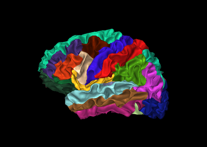
snap1 — With Parcellation Annotation

annot accepts a FreeSurfer .annot file and colors each vertex by its parcellation label. This example uses the DKTatlas parcellation.

img = snap1(
    lh_white,
    annot=lh_annot,
    bg_map=lh_curv,
)
display(img)

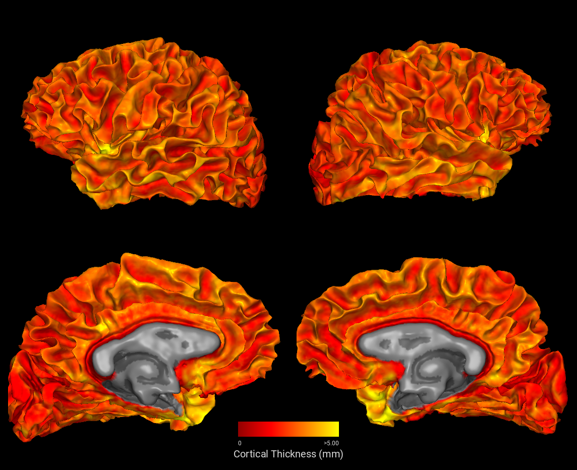
snap4 — Four-View Overview

snap4 renders lateral and medial views of both hemispheres and stitches them into a single composed image. Here we color both hemispheres by cortical thickness, masked to the cortex label.

from whippersnappy import snap4

img = snap4(
    sdir=sdir,
    lh_overlay=lh_thickness,
    rh_overlay=rh_thickness,
    colorbar=True,
    caption="Cortical Thickness (mm)",
)
display(img)

plot3d — Interactive 3D Viewer

plot3d creates an interactive Three.js/WebGL viewer that works in all Jupyter environments. You can rotate, zoom, and pan with the mouse. Requires pip install 'whippersnappy[notebook]'.

from whippersnappy import plot3d

viewer = plot3d(
    mesh=lh_white,
    bg_map=lh_curv,
    overlay=lh_thickness,
)
display(viewer)

snap_rotate — Rotating 360° Animation

snap_rotate renders a full 360° rotation of the surface. We output an animated GIF so it displays inline in all Jupyter environments including PyCharm. Use .mp4 as outpath instead for a smaller file when playing outside the notebook. This cell takes the longest to run — execute it last.

import os
import tempfile

from IPython.display import Image

from whippersnappy import snap_rotate

_gif_fd, outpath_gif = tempfile.mkstemp(suffix=".gif")
os.close(_gif_fd)

snap_rotate(
    mesh=lh_white,
    outpath=outpath_gif,
    overlay=lh_thickness,
    bg_map=lh_curv,
    roi=lh_label,
    n_frames=72,
    fps=24,
    width=800,
    height=600,
)

'/tmp/tmp5j860e5z.gif'

display(Image(filename=outpath_gif))
os.unlink(outpath_gif)